6 Linear models
- Chapter 5 introduced Darwin’s maize data, and the manual calculation of confidence intervals (CIs)
- In this chapter, the author discusses more efficient methods of calculating CIs
6.1 Introduction
install.packages("DAAG", repos = "https://cran.us.r-project.org")
install.packages("ggfortify",  repos = "https://cran.us.r-project.org")
install.packages("SMPracticals",  repos = "https://cran.us.r-project.org")
install.packages("ggplot2",  repos = "https://cran.us.r-project.org")
install.packages("arm",  repos = "https://cran.us.r-project.org")
install.packages("reshape2",  repos = "https://cran.us.r-project.org")
install.packages("tidyverse", repos = "https://cran.us.r-project.org")6.2 A linear model analysis for comparing groups
- The general function for creating linear models is
lm() - It’s good practice to assign a model to an object (i.e. ls0)
- Short for least squares model 0 because the linear model analysis uses a technique known as least squares
Create first model:
ls0 <- lm(formula = height ~1,  #the 1 indicates that we just want to
                                  #estimate an intercept
data = darwin) - ls0 is a model of height in relation to 1 (not another variable)
- When no comparisons are made in the model the intercept equals the grand mean
Generate a concise summary (table of coefficients) of key output of linear models:
display(ls0) #from the arm package
#> lm(formula = height ~ 1, data = darwin)
#>             coef.est coef.se
#> (Intercept) 18.88     0.58
#> ---
#> n = 30, k = 1
#> residual sd = 3.18, R-Squared = 0.00- display(ls0) output:
- coeff.est = the intercept (it’s the grand mean in this case)
- coeff.se = the standard error
- n = sample size
- k = # of parameters estimated by the model (in this case it’s 1 since it’s just the grand mean)
- residual sd = the SD of the heights of all 30 plants
- R-squared 0.00 = 0% of the variation in the data is accounted for by the explanatory variable since there is no explanatory variable, the proportion is 0%
The intercept is the grand mean of all of the Darwin maize data. Confirmation:
x<-format(round(mean(darwin$height), 2), nsmall = 2)
x <- as.numeric(x)
x
#> [1] 18.88
Visualize the data:
base_plot <- ggplot(darwin, aes(x = type, y = height)) + geom_boxplot() +
    theme_bw()
base_plot # the marked points are outliers 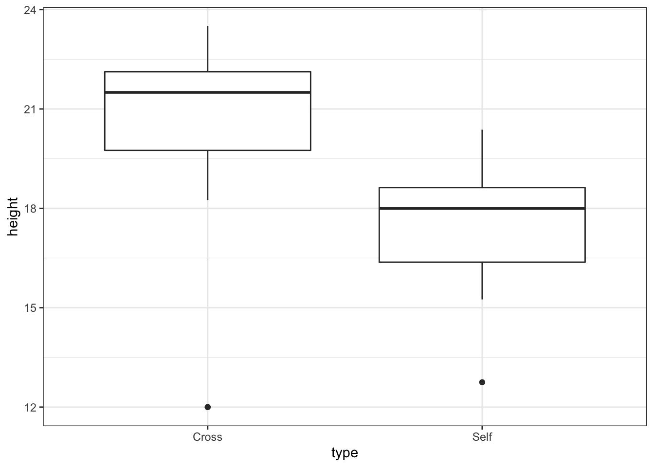
Create model of height by pollination type:
ls1 <- lm(height ~ type, data = darwin) #does height vary as a function of type of pollination? Summarize the model ls1:
display(ls1)
#> lm(formula = height ~ type, data = darwin)
#>             coef.est coef.se
#> (Intercept) 20.19     0.76
#> typeSelf    -2.62     1.07
#> ---
#> n = 30, k = 2
#> residual sd = 2.94, R-Squared = 0.18- display(ls1) output:
- Need to figure out what “Intercept” is in the table of coefficients
- It is no longer equal to the grand mean
- There are two levels encompasses in the explanatory variable “type”
- One is “self” and is listed as typeSelf
- So the intercept must be the other explanatory variable (cross)
- Also, R lists levels in alphabetical order (cross before self)
- In the table, the coeff.est of the intercept is the average height of cross pollinated progeny
- coef.se of the Intercept is the SE of the mean
- The coeff.est of typeSelf is the difference in mean height of the cross pollinated and self pollinated progeny (that’s why it is negative)
- This will help us answer the question, Is there any difference in plant height that results from the different pollination treatments?
- The coeff.se for typeSelf is also something new:
- It’s the standard error of the difference
- Variation expected around the difference
- The linear model calculates a pooled variation across all groups to take advantage of the fuller sample (greater n)
- Assumes that the groups have the same variance; this assumption must be checked
- residual sd - square root of the residual error variance
- R-squared - 18% of the variation is explained by the pollination variable
- Need to figure out what “Intercept” is in the table of coefficients
Annotate mean on scatterplot:
ggplot(darwin, aes(x = type, y = height)) + geom_point() +
  stat_summary(fun = mean, #superimpose the mean on the plot
               geom = "point",
               colour = "blue", shape =8, size =5)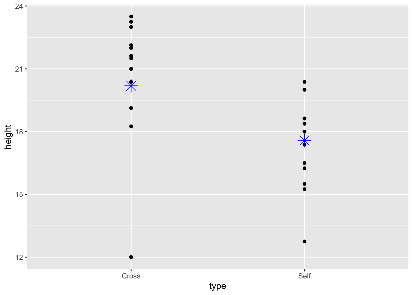
6.3 Standard error of the difference
- Standard error of the difference (SED) - standard error of the difference between two means:
- The subscripts indicate there are two groups (i.e. treatment groups)
6.4 Confidence intervals
Calculate upper and lower bounds of the CI for the model:
CI_ls1<-confint(ls1)
CI_ls1
#>                2.5 %     97.5 %
#> (Intercept) 18.63651 21.7468231
#> typeSelf -4.81599 -0.4173433- Output:
- Similar output to the
display()function - The first row (the Intercept) shows the 95% CI for the height of the seed developed from outcrossing
- The second row shows the 95% CI for the difference in height between the two groups
- Similar output to the
- The upper (97.5%) and lower (2.5%) bounds are percentiles of the normal distribution
- Helpful to incorporate all the data into one table:

- Darwin hypothesized that progeny produced through selfing would have lower fitness levels (reflected in height)
- CIs can be used to figure out if this is reflected in the data
6.5 Answering Darwin’s question
- The null hypothesis in this experiment is that there is no difference in fitness (height) of the progeny produced through selfing or outcrossing
- A confidence interval test can be used to uphold or reject the null hypothesis
- This requires that we determine if the predicted null value (zero) lies inside the confidence interval (see figure 5.3)
- If zero lies outside these bounds, then the null hypothesis can be rejected at that confidence interval because the estimated mean difference (-2.62 inches) can be distinguished from the null predicted value given the variability in the data
- Variability in the data is quantified through the standard error, which is used to calculate the CI
- We can visualize this on a numberline
Plot a number line with difference of means and its respective CI: (see guide)
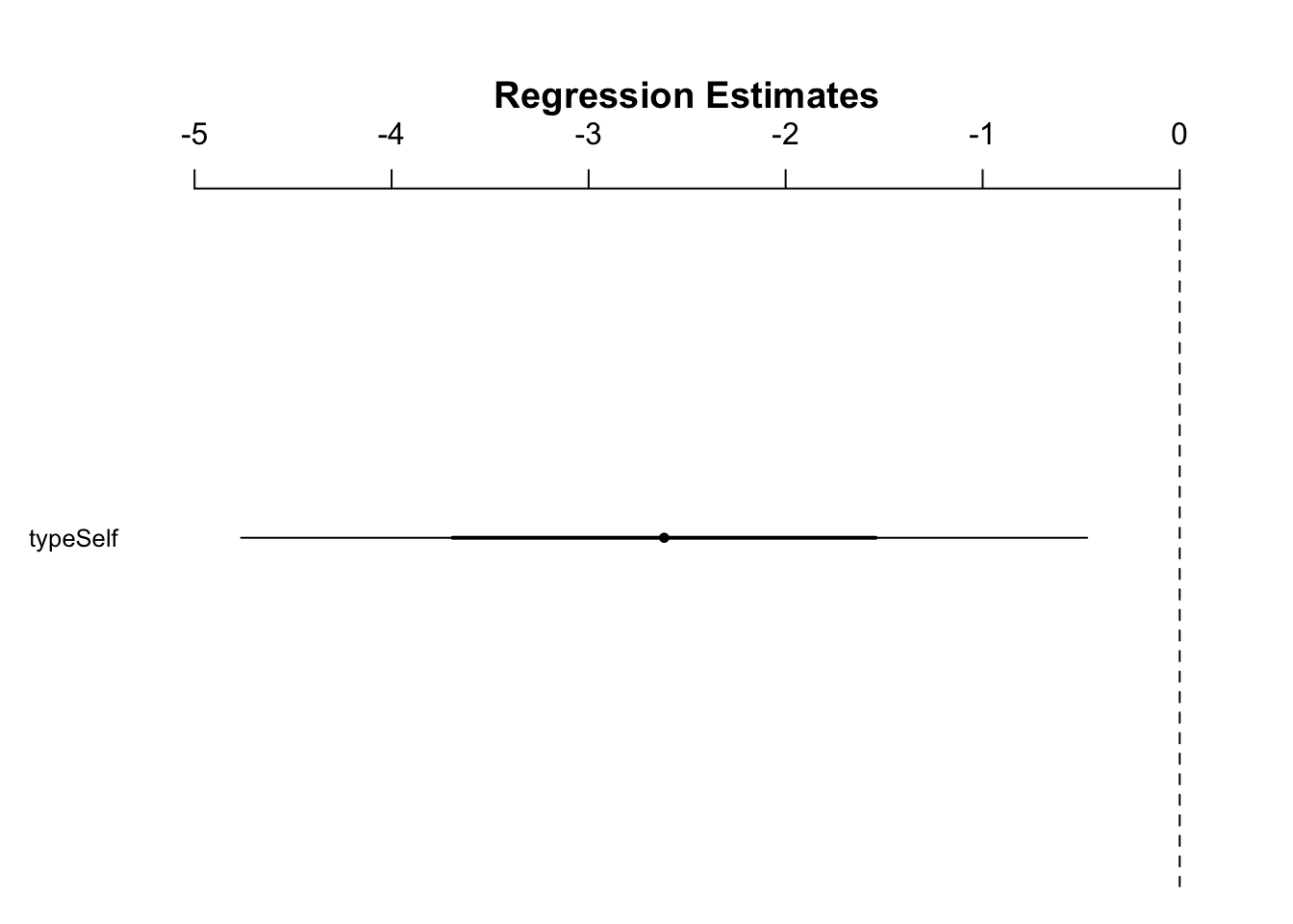
- Number line conclusions:
- since 0 is outside the 95% CI, we can reject the null hypothesis at this standard
Create a model with a 99% CI requirement:
confint(ls1, level = 0.99)
#>                 0.5 %     99.5 %
#> (Intercept) 18.093790 22.2895433
#> typeSelf -5.583512 0.3501789- Output:
- note the change in sign in the upper bound of typeSelf shows that 0 is now within the CI
Redraw the number line with the new model:
fig6_5 <- coefplot(ls1,
sd = 3) #sd actually refers the # of standard errors here 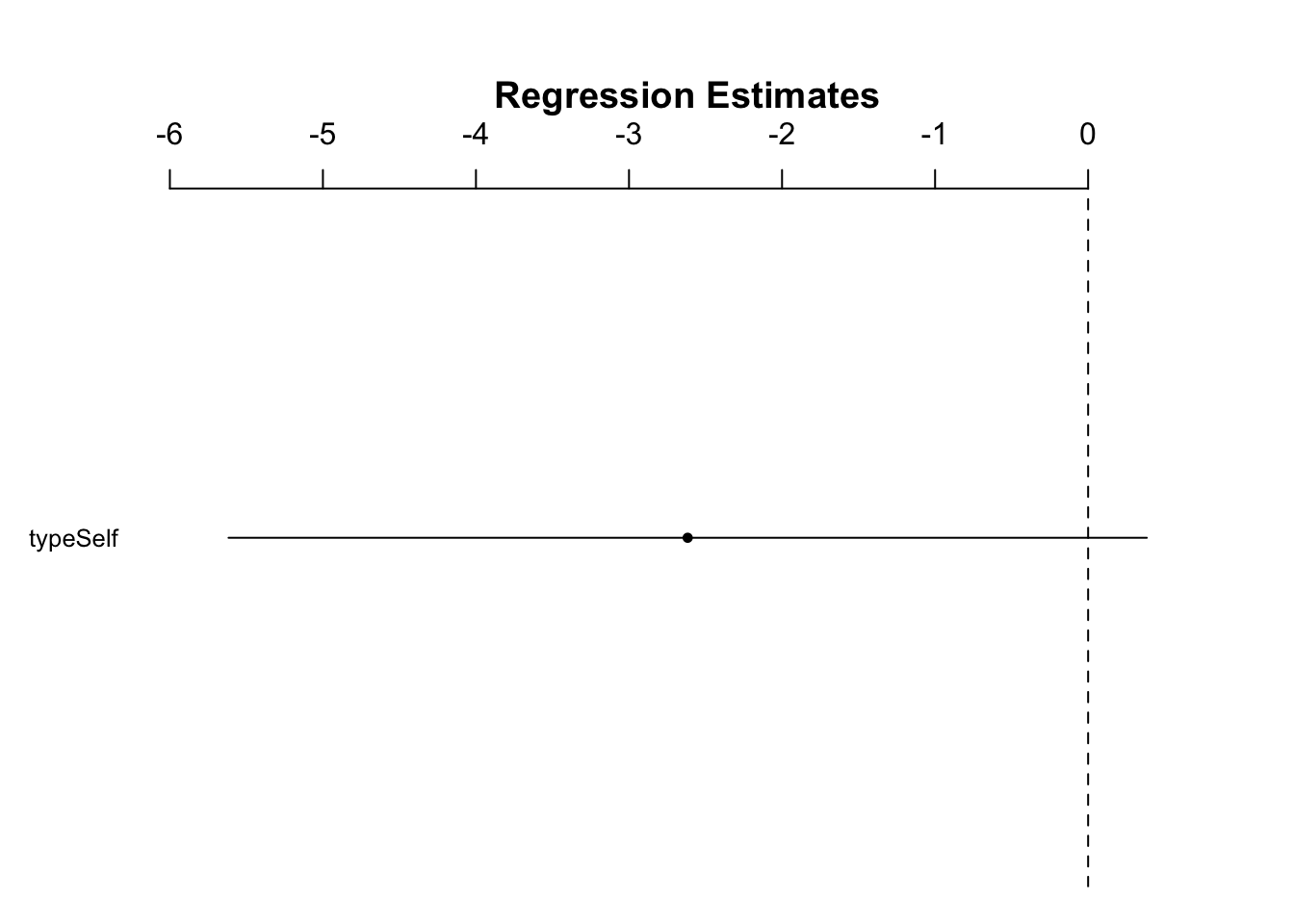
- Conclusions:
- cannot reject the null hypothesis at a 99% CI as 0 is within it
6.6 Relevelling to get the other treatment mean and standard error
- A limitation of these methods is that the table of coefficients from
display()will not produce the mean and standard error for another level- As we have seen, you can only get the difference of means and the SED
- To find the mean and standard error for the other level(s), the variables have to be relevelled
Relevel to get the mean and standard error data for the selfed progeny population:
darwin$type <- relevel(darwin$type, #in this column:
                       ref = "Self") #make the reference the Self group
Summarize the model:
display(lm(height ~type, data = darwin)) #now, Intercept's coef.est and coef.se refer to those of the selfed population
#> lm(formula = height ~ type, data = darwin)
#>             coef.est coef.se
#> (Intercept) 17.58     0.76
#> typeCross    2.62     1.07
#> ---
#> n = 30, k = 2
#> residual sd = 2.94, R-Squared = 0.18- The standard error of the mean (Intercept$coef.se) is the same for typeSelf as for typeCross (0.76)
- Based on the formula for SE, SE value depends on \(variance^2\) and the sample size (n) for each group
- However, R’s
lm()function uses a single (pooled) estimate of the residual variance for all treatment levels (this concept will be revisited in the ANOVA section) - So if the SEMs for different treatments vary, then it must be due to the sample size in each group differing
- But in the case of Darwin’s maize data, each group was comprised of 15 plants
- Since both groups had an equal number of biological reps and the
lm()was used, then we didn’t have to relevel the groups because we could have already known that the SEMs of the groups would be the same
6.7 Assumption checking
- The objective here is to assess that the assumptions that the unexplained variations in the two treatment groups are approximately normal are are equal in their variability
- It is recommended to plot the residual differences to assess this
- Residuals are the differences between the observed values (heights) and the ‘fitted’ values which are predicted by the linear model
- This assumption of approximate normality applies here because linear models use the normal distribution as a model for the variabiliity
- This is where measures of precision (SEs) and confidence (CIs) are derived from
- The assumption of approximately equal variance follows from the use of a single pooled estimate of variance across all treatment groups
6.7.1 Normality
- Check assumptions using the diagnostic plots using ggfortify -
- Display the normal quantile (Q-Q) plot:
fig6_6 <- autoplot(ls1,
                   which = c(2), #refers to which of the graphs you want displayed
                                      #in this case it's it can be c(1,2,3,4)
                   ncol = 1) #sets the orientation in which the plots are displayed
fig6_6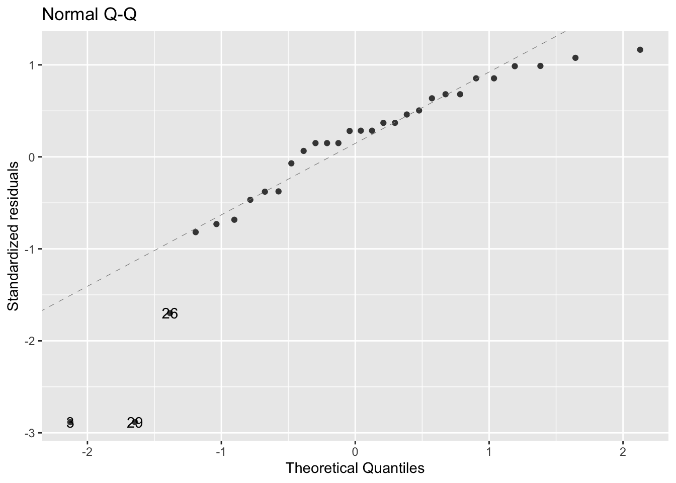
- fig6_6 takeaways:
- This plot graphs the quantiles of the distribution of the residuals compared to the quantiles of a random sample of normally distributed numbers
- The dotted diagnonal line represents that normal distribution
- When most of the dots fall around the dotted line, they closely match the normal model
- A large portion of the residuals are approximately normally distributed
- The points that deviate from normal are at the extremes
- This is not a surprise because we already know there are outliers in the data
- Overall, this assessment shows that data are not ideally normal, but not appropriate still
6.7.2 Equal variance
- Two graphs to assess if the variances in the treatment groups are approximately equal:
- Raw residuals plot (left) - positive and negative values
- Standarized residuals plot (right) - positive values
- \(\sqrt|\frac{residuals}{residuals.SD}|\)
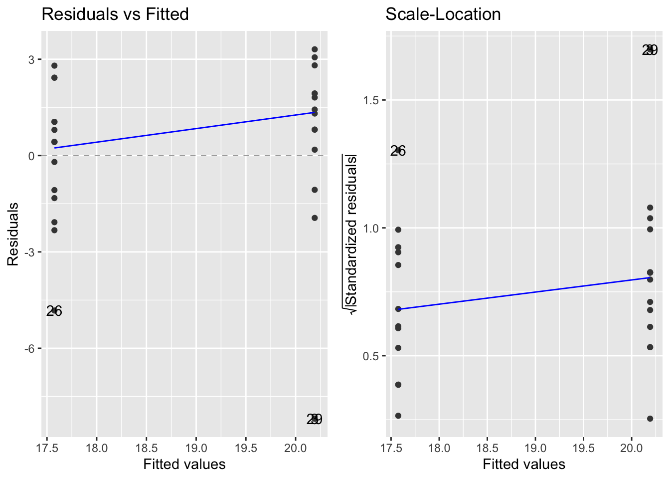
- fig6_7:
- The group with the higher fitted values is the outcrossed group, which has a higher mean height
- These plots confirm our impressions of the raw data (see base_plot) that the cross pollinated treatment data are more variable, mainly due to the outlier values
Appendix 6b: Robust linear models
Robust linear model function (rlm()):
summary(rlm(height ~ type, data = darwin))
#>
#> Call: rlm(formula = height ~ type, data = darwin)
#> Residuals:
#>     Min      1Q  Median      3Q     Max
#> -9.1542 -1.4374  0.2501  0.9469  2.6251
#>
#> Coefficients:
#>             Value   Std. Error t value
#> (Intercept) 17.7499  0.6362    27.8989
#> typeCross    3.4043  0.8998     3.7836
#>
#> Residual standard error: 1.646 on 28 degrees of freedom
Appendix 6c: Exercise
Repeat analysis with Darwin’s mignonette data…
str(mignonette)
#> 'data.frame':    24 obs. of  2 variables:
#>  $ cross: num  21 14.2 19.1 7 15.1 ...
#> $ self : num 12.9 16 11.9 15.2 19.1 ...- mignonette data is in wide form, but I want to make the pollination type a variable
Add two variables for the pollination type:
mignonette$type1 <- "type_cross"
mignonette$type2 <- "type_self"
head(mignonette)
#>    cross   self      type1     type2
#> 1 21.000 12.875 type_cross type_self
#> 2 14.250 16.000 type_cross type_self
#> 3 19.125 11.875 type_cross type_self
#> 4  7.000 15.250 type_cross type_self
#> 5 15.125 19.125 type_cross type_self
#> 6 20.500 12.500 type_cross type_self
Combine type1 and type2 variables into one new column - type:
df.new<-melt(mignonette, id.var = c('type1','type2'), variable.name = 'type')
head(df.new)
#>        type1     type2  type  value
#> 1 type_cross type_self cross 21.000
#> 2 type_cross type_self cross 14.250
#> 3 type_cross type_self cross 19.125
#> 4 type_cross type_self cross  7.000
#> 5 type_cross type_self cross 15.125
#> 6 type_cross type_self cross 20.500
Subset this dataframe and change one of the variable names:
mignonette2 <- subset(select(df.new, -type1 & -type2))
head(mignonette2)
#>    type  value
#> 1 cross 21.000
#> 2 cross 14.250
#> 3 cross 19.125
#> 4 cross  7.000
#> 5 cross 15.125
#> 6 cross 20.500

mignonette2$height <- mignonette2$value
head(mignonette2)
#>    type  value height
#> 1 cross 21.000 21.000
#> 2 cross 14.250 14.250
#> 3 cross 19.125 19.125
#> 4 cross  7.000  7.000
#> 5 cross 15.125 15.125
#> 6 cross 20.500 20.500
Create scatter plot:
base_plot<-ggplot(mignonette2, aes(x = type, y = height)) +
  geom_boxplot() +
  theme_bw()
base_plot # there are no outliers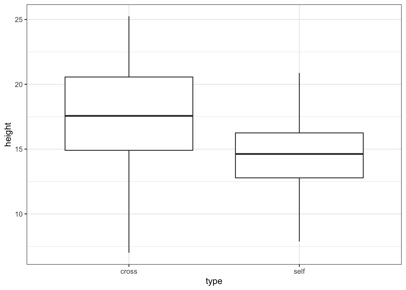
Change height to numeric object:
mignonette2$height <- as.numeric(mignonette2$height)
str(mignonette2)
#> 'data.frame':    48 obs. of  3 variables:
#>  $ type  : Factor w/ 2 levels "cross","self": 1 1 1 1 1 1 1 1 1 1 ...
#>  $ value : num  21 14.2 19.1 7 15.1 ...
#>  $ height: num  21 14.2 19.1 7 15.1 ...
Use wide-format dataframe now for some calculation:
mignonette$difference <- mignonette$cross - mignonette$self Calculuate mean, SD, and standard error:
Create linear model:
mig_ls <- lm(value ~ type,data = mignonette2)Summarize the mig model:
display(mig_ls)
#> lm(formula = value ~ type, data = mignonette2)
#>             coef.est coef.se
#> (Intercept) 17.18     0.82
#> typeself    -2.56     1.16
#> ---
#> n = 48, k = 2
#> residual sd = 4.00, R-Squared = 0.10
Calculate 95% CI for the model:
confint(mig_ls)
#>                 2.5 %     97.5 %
#> (Intercept) 15.531838 18.8223283
#> typeself    -4.884019 -0.2305639
Plot model on a number line:
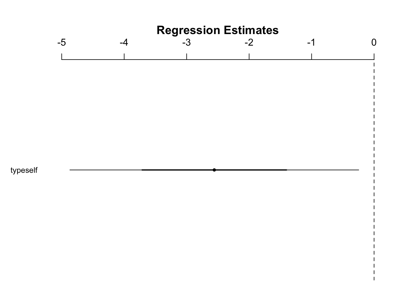
- CI does not contain zero, we can reject the null hypothesis at a 95% CI
Now create model at a 99% CI:
confint(mig_ls, level = 0.99)
#>                0.5 %     99.5 %
#> (Intercept) 14.98085 19.3733201
#> typeself -5.66324 0.5486562- now the 99% CI does contain zero, so we will fail to reject the NH at this level
Check some diagnostics, starting with the normal q-q plot:
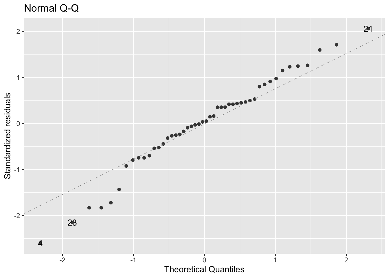
- since most of the points are on or near the dotted line, the data seem to fit the model appropriately
Next, the residual variance plots:
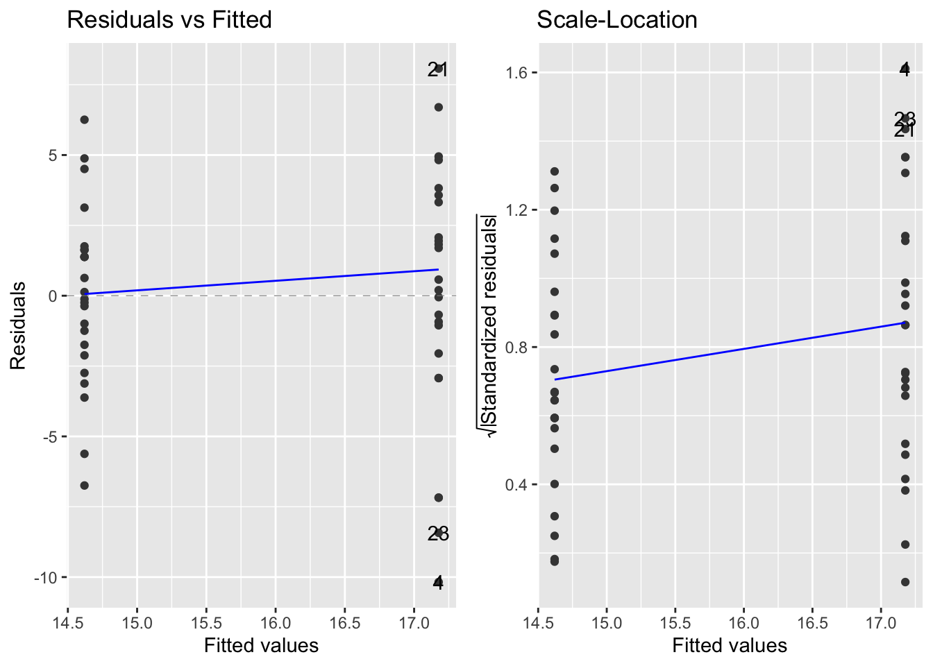
- the variances look comparable