9 Testing

9.1 Significance testing: Time for t

Statisticians think that the overfixation on p-values has contributed to the reproducibility crisis in science
That’s why the author’s focus of this text is on estimation, which relies on estimates and confidence intervals
This chapter introduces the Student’s t-test which will generate a p-value

install.packages("arm",  repos = "https://cran.us.r-project.org")
install.packages("ggplot2",  repos = "https://cran.us.r-project.org")
install.packages("Sleuth2",  repos = "https://cran.us.r-project.org")
install.packages("SMPracticals",  repos = "https://cran.us.r-project.org")

library(arm)
library(ggplot2)
library(Sleuth2)
library(SMPracticals)

9.2 Student’s t-test: Darwin’s maize

The Student’s t-test
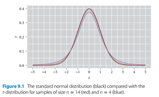
- Uses the t-distribution
  - This is like a small sample size version of the normal distribution
- There are two basic forms a t-test can take:
  - The one sample t-test takes the mean of a sample and compares it with a null hypothesis of zero
  - The two sample t-test compares the difference between the means of two samples against a null a hypothesis of no difference (zero)
    - The paired two sample t-test is a subtype that applies when the values of two samples come in pairs (like in the darwin maize data)
- R has a function for the t-test but the author tends to avoid it. Criticism from the author about the default R t-test:
  - the parts of the t-test include:
    - a difference
    - its standard error (and the CI used to calculate it)
    - the observed value of t
    - the critical value of t
    - the degrees of freedom
    - the P-value
  - the default R t-test output is poorly ordered and missing some of this information
  - the default is not the classic t-test but another variant called Welch’s
    - Welch’s might be good for research since it doesn’t assume equal variance though
  - but adds another twist so it’s not appropriate for teaching beginners
the general form of a t-test is:

\(observed \;t = \frac{difference}{SE}\)

this is a more formal version of what was done in earlier chapters in which the output of the display() function - the estimates and the standard errors were compared
as a rule of thumb/eyeball test, the estimate should be twice as large as its standard error to reject the null hypothesis at the lowest level of confidence (95%) and three times as large for the next level (99% CI) and so on
when sample sizes are larger, t converges to the normal distribution
when sample sizes are smaller, the t distribution is shorter and wider than normal

two t values of the t-test:
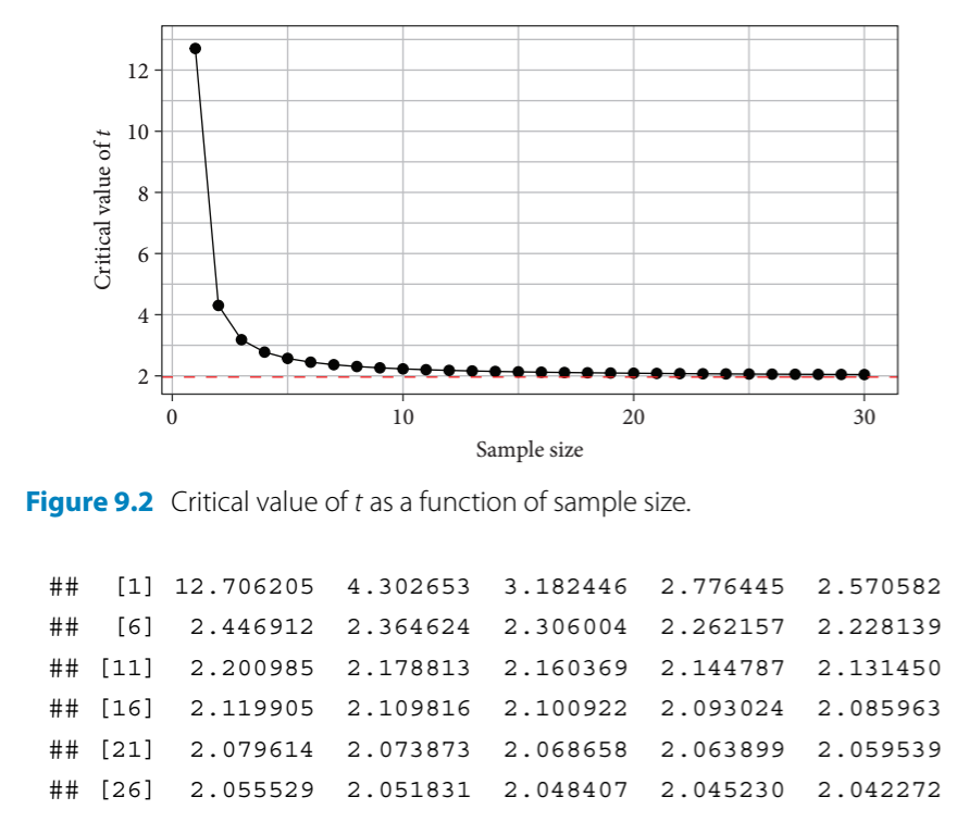
- critical t value - sets the bar for comparison - this is the minimum t value required to achieve a given level of significance (P = 0.05, 0.01, etc.)
- observed t value - calculated by dividing the estimate by its standard error
  - if the observed t value is larger than the critical t value, then the result is declared significant at that level

For performing a paired t-test with darwin’s maize data, the observed t value must be compared to the critical value with the corresponding critical t value for the sample size that Darwin had (\(n = 15 \;pairs\))

Calculate the critical t value when P = 0.05 and n = 15 pairs:

qt(0.975, df = 14)  #mean + 2SEs; 0.975 is the upper CI limit for a 95% CI 
#> [1] 2.144787

Summarize the model for a version of the maize data that omits the pairing aspect (for standard two sample t-test):

summary(
  lm(height ~ type, data = darwin)) #this linear model omits the pairing aspect 
#> 
#> Call:
#> lm(formula = height ~ type, data = darwin)
#> 
#> Residuals:
#>     Min      1Q  Median      3Q     Max 
#> -8.1917 -1.0729  0.8042  1.9021  3.3083 
#> 
#> Coefficients:
#>             Estimate Std. Error t value Pr(>|t|)    
#> (Intercept)  20.1917     0.7592  26.596   <2e-16 ***
#> typeSelf     -2.6167     1.0737  -2.437   0.0214 *  
#> ---
#> Signif. codes:  
#> 0 '***' 0.001 '**' 0.01 '*' 0.05 '.' 0.1 ' ' 1
#> 
#> Residual standard error: 2.94 on 28 degrees of freedom
#> Multiple R-squared:  0.175,  Adjusted R-squared:  0.1455 
#> F-statistic:  5.94 on 1 and 28 DF,  p-value: 0.02141

summary() takeaways:
- The second row of the coefficients table tests the null hypothesis by comparing the observed difference in height between progeny of selfed and cross pollinated plants (-2.6167)
- The first row tests the mean height of the cross pollinated plants versus a null hypothesis of an average height of zero
  - This was not a comparison we intended to make in advance or really at all
It can be beneficial to specify only the tests we want to have run even if it means more typing
The average difference in height is -2.6167 and its standard error of the difference is 1.0737

This produces an observed t value of:

-2.6167/1.0737 #difference/standard error of the difference 
#> [1] -2.437087

critical t value for this data is 2.144787
observed t value for the data is -2.437087

It is better/more informative to work with CIs:

confint(lm(height ~ type, data = darwin))
#>                2.5 %     97.5 %
#> (Intercept) 18.63651 21.7468231
#> typeSelf    -4.81599 -0.4173433

Again, this 95% CI does not encompass 0; therefore, the null hypothesis can be rejected at this level
In the previous summary() chunk, the standard two sample t-test was performed without factoring in the pairing

Generate table of coefficients for a paired t-test:

summary(lm(height ~ type + pair, data = darwin))
#> 
#> Call:
#> lm(formula = height ~ type + pair, data = darwin)
#> 
#> Residuals:
#>     Min      1Q  Median      3Q     Max 
#> -5.4958 -0.9021  0.0000  0.9021  5.4958 
#> 
#> Coefficients:
#>             Estimate Std. Error t value Pr(>|t|)    
#> (Intercept)  21.7458     2.4364   8.925 3.75e-07 ***
#> typeSelf     -2.6167     1.2182  -2.148   0.0497 *  
#> pair2        -4.2500     3.3362  -1.274   0.2234    
#> pair3         0.0625     3.3362   0.019   0.9853    
#> pair4         0.5625     3.3362   0.169   0.8685    
#> pair5        -1.6875     3.3362  -0.506   0.6209    
#> pair6        -0.3750     3.3362  -0.112   0.9121    
#> pair7        -0.0625     3.3362  -0.019   0.9853    
#> pair8        -2.6250     3.3362  -0.787   0.4445    
#> pair9        -3.0625     3.3362  -0.918   0.3742    
#> pair10       -0.6250     3.3362  -0.187   0.8541    
#> pair11       -0.6875     3.3362  -0.206   0.8397    
#> pair12       -0.9375     3.3362  -0.281   0.7828    
#> pair13       -3.0000     3.3362  -0.899   0.3837    
#> pair14       -1.1875     3.3362  -0.356   0.7272    
#> pair15       -5.4375     3.3362  -1.630   0.1254    
#> ---
#> Signif. codes:  
#> 0 '***' 0.001 '**' 0.01 '*' 0.05 '.' 0.1 ' ' 1
#> 
#> Residual standard error: 3.336 on 14 degrees of freedom
#> Multiple R-squared:  0.469,  Adjusted R-squared:  -0.09997 
#> F-statistic: 0.8243 on 15 and 14 DF,  p-value: 0.6434

New table of coefficients output:
- Takes the crossed plant from pair 1 as the intercept
- Shows the mean difference in height of the crossed plants (-2.6167)
- Then shows the average difference of each pair relative to pair 1
Ignore these differences of pairs and see that the second row gives us the t value for the paired t-test:

-2.6167/1.2182
#> [1] -2.148005

This is the observed t value, which is way smaller than the critical t value (2.144787)
This finding corresponds to the large p value in the table which is 0.6434

We can use a the linear model function to perform the equivalent of a one-sample t test: - generate a single sample of differences:

ex0428$Difference <- ex0428$Cross - ex0428$Self

Fit a linear model that only estimates the mean difference:

summary(lm(Difference ~1, #the 1 indicates the intercept, which is the mean of a single sample of differences
           data = ex0428))
#> 
#> Call:
#> lm(formula = Difference ~ 1, data = ex0428)
#> 
#> Residuals:
#>      Min       1Q   Median       3Q      Max 
#> -10.9917  -1.2417   0.3833   3.0083   6.7583 
#> 
#> Coefficients:
#>             Estimate Std. Error t value Pr(>|t|)  
#> (Intercept)    2.617      1.218   2.148   0.0497 *
#> ---
#> Signif. codes:  
#> 0 '***' 0.001 '**' 0.01 '*' 0.05 '.' 0.1 ' ' 1
#> 
#> Residual standard error: 4.718 on 14 degrees of freedom

9.3 Summary: statistics

Alternate source on t-tests
I will probably rarely if ever use a one sample t-test
use two-tailed t-test since we don’t need to determine the direction of the difference
use a paired t-test if the groups come from a single population
- i.e. if you are measuring gene expression in two groups of cannabis plants over time or before/after methyl jasmonate treatment
use a two sample (unpaired) t-test if the two groups come from different populations
- i.e. comparing some feature of two varieties of P. cubensis
- if they are different, then the CI will not include 0 so the null hypothesis can be rejected

8 Prediction

10 Intervals